
While on a run yesterday in my new Xero brand running sandals[1], I found myself thinking about the proposal I have to write for marine geochemistry. Since I have read a fairly comprehensive assortment of water column particle flux papers, I figure it might be a good fit for this proposal. Vertical carbon flux, which is mediated by particles, form the link between the water column and sedimentary carbon deposits. The quality and quantity of these particles should, to first order, estimate carbon burial to the seafloor.
So for this proposal, I want to write a particle flux model to estimate the impact of aggregation and disaggregation on to carbon burial. So let’s get started.
Particles
Starting out, it seems obvious that if this is going to be a individual-based model, I better have some particle object. Particles within the water column have a vast array of features[2], but to keep it simple these particles will include: mass, radius (ESD), density, age. Furthermore, some derived qualities will include sinking velocity and an ability to decay (lose mass).
The particle size spectrum has become a hot topic in carbon cycling due to the recognition that the size of a particle influences sinking speed dramatically and that technology now allows to measure particle sizes in situ. Our current understanding is that the particle size spectrum fits a log-normal distribution ranging from 0.2 $\mu$m to >1 cm or a source distribution of -6 to -2 (see appendix for details).
The sinking velocity of a particle can be calculated from Stokes Law which says
$$v = \frac{2}{9} \frac{(\rho-\rho_{ref})}{\mu}g r^2$$
where $\mu$ is the dynamic viscosity of the water (assumed to be 1.519 here), $g$ is the acceleration due to gravity, and $\rho$ and $rho_{ref}$ is the density of the particle and water respectively. For the time being, we’ll assume that particles have a constant density of $1.100 kg m^{-3}$ and seawater has a density of $1.035 kg m^{-3}$.
The radius (or equivalent spherical diameter as it is commonly called)[3] is a simple function of mass and density.
$$\frac{4}{3}\pi r^3 = \frac{m}{\rho}$$
So far, here is our particle class which includes all the above with the addition of an update() method to allow the depth to change (i.e. velocity x time) as well as for decay (1% decay per hour).
rho_ref = 1.035
mu = 1.519

class Particle:

    mass = 0 # kg
    radius = 0 # m
    depth = 0 # m
    density = 0 # kg / m^3
    velocity = 0 # m/s
    age = 0

    def __init__(self, mass, radius, depth):
        self.mass = mass
        self.radius = radius
        self.depth = depth
        self.density = self.mass / (4.0/3.0 * 3.14159 * (self.radius)**3)
        assert(self.density - rho_ref > 0)
        assert(self.radius > 0)
        self.set_velocity()
        assert(self.velocity > 0)

    def set_velocity(self):
        self.velocity = 2.0 / 9.0 * (self.density - rho_ref) * 10 * self.radius**2

    def __str__(self):
        return "Particle of mass " + str(self.mass)

    def update(self, dt):
        self.depth = self.depth + dt*self.velocity
        self.age += 1

    def decay(self, dt):
        self.mass *= (0.99)**(dt/3600)
        self.radius *= 0.99**(0.333333*dt/3600)
        self.set_velocity()

    def members(self):
        return(1)
Aggregation
In order to allow the particles to aggregate, we need a way to organize particles into aggregates; but this will not be too hard if we simply start with our particle class from above. Aggregates have all the same features of particles with one additional property: they are made up of particles. To represent this aspect, let’s construct aggregates from existing particles (they can’t simply come into existence after all). On top of this, we’ll give aggregates the ability to add particles to themselves and to adjust their properties accordingly.
When we add a particle to an aggregate, the mass should be conserved, the radius should increase, and the density should stay the same (at least in the simplest model). So the methods will simply need to be adapted for the new aggregate object we have.
The aggregate process within the water column is not uni-directional, so our aggregate object should also be able to handle the disaggregation process quite naturally. Beyond that, the aggregate class is pretty much all set.
class Aggregate:
    part = [] # List of particles
    dim = 2
    depth = 0 # m
    density = 0 # kg/m^3
    radius = 0 # m
    velocity = 0 # m/s
    mass = 0 # kg
    age = 0

    def __init__(self, p):
        self.part = [p]
        self.depth = p.depth
        self.mass = p.mass
        self.density = 3.0 * p.mass / 4.0 / 3.14159 / (p.radius)**3
        self.set_radius()
        self.set_velocity()

    def dis(self):
        for i in range(len(self.part)):
            self.part[i].depth = self.depth
        return(self.part)

    def add(self, idd):
        self.part.append(idd)
        self.set_radius()
        self.set_density()
        self.set_velocity()
        self.mass += idd.mass
        assert(self.density - rho_ref > 0)
        assert(self.radius > 0)

    def set_radius(self):
        vol = sum([4.0*3.14159/3.0 * i.radius for i in self.part])
        self.radius = vol**(1/self.dim)

    def set_density(self):
        #self.density = self.mass / (4.0/3.0 * 3.14159 * self.radius**self.dim)
        self.density = 1.1

    def set_velocity(self):
        self.velocity = 2.0 / 9.0 * (self.density - rho_ref) * 10 * self.radius**2

    def __str__(self):
        return(str([i.__str__() for i in self.part]))

    def set_mass(self):
        self.mass = sum([i.mass for i in self.part])

    def decay(self):
        for i in range(len(self.part)):
            self.part[i].decay()

    def update(self, dt):
        self.depth = self.depth + dt*self.velocity # Sink
        self.age += 1 # Age
        for i in range(len(self.part)): # Decay
            self.part[i].decay()
        self.set_mass()
        self.set_radius()
        self.set_velocity()

    def members(self):
        return(sum([i.members() for i in self.part]))
Model Environment
Now that we have the particle and aggregate objects, the environment in which they exist needs to be created. While this may, at first glance, seem like the easy part, the reality is that it is the parameterization of the environment that we know the least about[4].
The first step is deciding how the particles are to aggregate. The simplest choice will say that when particles physically make contact (i.e. when one particle is within the radius of another particle) that they aggregate. An additional parameter that feels a bit more natural would be to allow particles to hit yet not aggregate some of the time. We can do that with the following code.
## Test for contact
if ( (depth_1 - depth_2)^2 < (r_1 + r_2)^2 ):
    if (random.random() < p_agg):
        ## For aggregate
    else:
        #Do nothing
Here p_agg is the probability that two particles will form an aggregate when they come together. In essence, this parameter controls how “sticky” the particles (and aggregates) are. If we wanted to we could allow this to change with depth or for the age of particles if we were interested in these effects (and had data to parameterize it with).
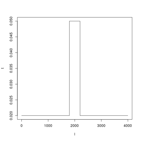
Since we are interested with depth-mediated dis-aggregation, we can use the same idea as above but without the test for collision. For now, I’ve decided that a delta-like function will be the best implementation based on my limited data.
def p_dis(d):
    if (d < 1800):
        return(0.02)
    if (d > 2200):
        return(0.02)
    return(0.05)
The resulting probabilities are:
Bringing it together
In bringing these pieces together, where are only a couple more things that need to be sorted out. Most critically, how do we efficiently test for particles that collide. We could run the test we wrote above between every two particles but this is far too inefficient to ever be in my code base ($O(N^2)$) so let’s find a more elegant solution.
To keep track of all the particles we have, we’ll have them in a list (which is certainly a strength of Python). This means that the list can be sorted with the built-in Timsort algorithm, which is generally quite efficient on real world, partially sorted data sets. To implement this, we just need to tell the sorting algorithm how to pull the data upon which it will sort.
def getKey(p):
    return(p.depth)
Can’t get much easier than this.
The plan now then, is to make a much of particles (which we’ve discussed before) throughout the photic zone (i.e. top 100 m of the water column) and then let them sink. We then sort them and test for aggregation/disaggregation. We can also say that at after a certain depth, they’ve hit the sea floor and will no longer sink or decay.
for tt in range(total):
    ## Update particles
    i=0
    while i < len(test):
        test[i].update(dt)
        if (test[i].depth > 3000):
            bottom.append(test[i])
            test.pop(i)
        else:
            i+=1

    mass.append(sum([i.mass for i in test]))
    test.sort(key=getKey)

    ## Run through aggregation/disaggregation tests
    i = 0
    while i < len(test):
        ## test for aggregation
        if (random.random() < p_agg and i < len(test)-1):
            if ( (test[i].depth - test[i+1].depth)**2 < test[i].radius**2):
                test[i] = Aggregate(test[i])
                test[i].add(test[i+1])
                test.pop(i+1)
                i += 1

        ## test for disaggregation
        elif (random.random() < p_dis(test[i].depth) and test[i].members() > 1):
            piece = test[i].dis()
            for n in range(len(piece)):
                test.append(piece[n])
            test.pop(i)
        else:
            i+=1
We now have a functional model and can start adjusting parameters and developing diagnostics to understand the dynamics of particle aggregation. I’ll save all the results and discussion of the model for another article.
- Running sandals have been a great change for me and I should do a full write up sometime in the future.
- For example, particle features include mass, center of mass, moment of inertia, chemical functional groups, soluble fractions, porosity, density, shape, etc.
- The term Equivalent Spherical Diameter is used in allometry as a proxy for size when comparing two, differently shaped objects. For particles in the water we would use ESD but for the model we’re assuming spherical particles.
- Most of science is observational meaning that we can witness the impact of environment on the thing that we are interested about, and then we are forced to infer the cause and effect relationship. Within the water column we can see the attenuation of particles with depth, and so assume that particles are degraded over time; but we still understand very little about the underlying mechanisms and processes governing this observation.