Being able to appropriately address uncertainty and error is fundamental to the pursuit of science. Without it, results and theory would never match up since theory usually involves a level of abstraction that permits simplification of the problem and observational results are never perfect and include all sorts of uncertainty. Recently I’ve been trying to quantify and approximate the error terms for the data that powers my model.
The Philosophy
Most people envision that uncertainty metrics such as standard deviation or confidence intervals are those final pieces of the puzzle that scientists work on after all the ‘real’ science is over, but the truth is a bit less orderly. Statistics such as the ones I’ve mentioned must be appreciated even before the experiment or model even run. No matter what experiment or field you’re working in, the first step is always the same: figure out what outcomes are possible and to predict the outcome. Now I’m not saying to prejudge the outcome, but rather have an idea of what range of outcomes you are willing to accept.
You should expect very different results from mixing water and table salt than you would expect in mixing sodium metal and water, and that’s a good thing. Understanding the uncertainty, limitations and goals of the experiment are critical first steps for successful science.
The Work
While most of the work and analysis are dreadfully boring, but I want to include a sampling here anyway. In terms of tools, I suppose I should mention that I use a combination of Excel, R and scrap paper for all my error analysis. One of the best way’s I’ve found to rigorously and properly run an analysis for a small section of work is to write an R script that walks you through the analysis. By doing so I not only can easily cite where a particular number came from, but I can also remember how I did it exactly.
# Gun Clearence Rates -- see Dam and Peterson 1988 for data and formulae.
# This file: Thomas Bryce Kelly (2015)
#

## Data they present
temp = c(0,1,3,6,6,6.4,9,10,11.5,11.5,13,13,15,17) #temp = [C]
K = c(0.014,0.0065,0.016,0.018,0.024,0.031,0.033,0.038,0.026,0.035,0.041,0.044,0.039,0.035) # K = [min^-1]

## Log transform
K = log(K)

## Run linear regression (optional)
# lm = lm(lk~temp)

## Formula (3) from Table III (transformed)
y = 0.08643*temp-4.41694

## Use the SE of the residual to calculate 95% CIs
t = qt(0.95, length(temp)-2)
r = sqrt(sum((y-K)^2))
yu = (0.08643)*temp-4.41694+r/length(temp-2)*t
yl = (0.08643)*temp-4.41694-r/length(temp-2)*t

## Plot the Results
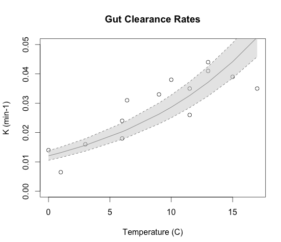
plot(temp,exp(K), ylim=c(0,0.05), xlab="Temperature (C)", ylab="K (min-1)", main="Gut Clearance Rates")
lines(temp, exp(y))
lines(temp, exp(yu), lty=2, col=rgb(0.2,0.2,0.2))
lines(temp, exp(yl), lty=2, col=rgb(0.2,0.2,0.2))
polygon(c(temp,rev(temp)),c(exp(yl),rev(exp(yu))), col=rgb(0.8,0.8,0.8,0.5), border=NA)
Not only does it provide me with excellent notes to refer too, but I can make nice images to go along with it:
