Believe it or not, but it is already the end of the semester for me and my peers. Somehow nearly four months have disappeared once again into that historical accident that we call the past. Since each of my three classes have required a project to be done for the final, I figure that I may as well adapt each of them here so I can share them with others.
For the first entry, here is my Marine Primary Productivity final which includes aspects of both the presentation as well as the paper.
Inverse Modeling: an exploration of the null space within a planktonic community
Introduction and Background
Although it is critically important in forming responsible management plans, interrogating and understanding ecological food webs is a notoriously difficult task (Raffaelli 2006). Often the nutrient flows are obscured by complex community dynamics that vary widely in both temporal and spatial scales. Compounding the uncertainty is a dearth of available metrics that are assailable to direct measurement. One such example might be the grazing rate of Microzoa (MIC) on Hetero Nanoflagellates (HNF). The overall MIC grazing rate can be readily assayed (Taniguchi et al.2012), but class specific rates are rarely interrogated in the field. Neither quantity can be measured in situ, which introduces further sources of error and another layer of assumption. Due to this complex topology and the dynamic nature of life, ecological food webs are difficult to quantify.
Marine plankton communities are even more difficult to process compared to their terrestrial doppelgangers due to the plethora of species and the relative scales (Nencioli et al. 2011)–both large in the case of the water column and small in the case of the phytoplankter–experienced by the oceanographer. Inverse modeling is one avenue of research that permits a deep integration of both the theory and the data (Oevelen et al. 2010).
Inverse modeling is a data regression technique where a set of structural and physical constraints are combined with field and laboratory data to render simulated ecosystem networks. An abundance of previous work has been done in both developing the methods (Stukel et al. 2012; Saint-Beat et al. 2013) as well as applying them to a variety of areas (Vezina and Piatt 1988; Richardson et al. 2004; Oevelen et al. 2010).
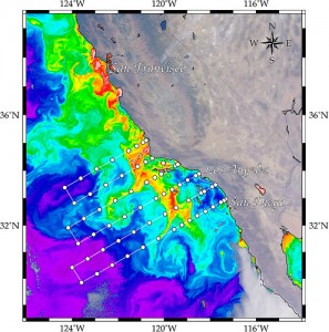
The California Current Ecosystem LTER (CCE LTER) is a study region in the coastal upwelling zone of the California current (Figure 1). Having it’s beginnings as the California Cooperative Oceanic Fisheries Investigations (CalCOFI) in 1949 (Ohman and Venrick 2003), the CCE LTER hosts reliable data sets for the past 65 years. The study area has changed over the years, but it has always focused on the waters from San Diego to San Fransisco and reaching out from shore to nearly 300 km. This region is highly variable in terms of productivity and community composition, and it has been studied extensively in terms of transport processes (Auad et al. 2011) and fisheries management (Field and Francis 2006; Coleman 2008). Nonetheless, an integration of the geophysical with that of the biological has remained elusive.
As an upwelling zone, the potential for massive carbon draw-down and sequestration to the sediments due to primary productivity is high. Yet the same processes that make the region particularly productive in terms of Chl a also obscure the efficiency of the biological pump.
An important focus of the CCE LTER since it’s official launch in 2004 is to identify and interrogate the abrupt and massive changes in community composition throughout time (Goericke and Ohman 2015). These abrupt and non-linear transitions in ecosystem composition are critical to formulating intelligent fishery management plans, yet the unlaying mechanisms remain elusive (Ohman 2004). Furthermore, the mechanisms and their dynamics may help reveal the impacts of climate change for this region (see Ohman et al. 2013 for an introduction). This project, in particular, aims to identify the community structure on a functional level while providing a common framework by which to understand the large-scale changes in community composition over both time and space.
Methods
To understand the validity of these assumptions, and to further build a foundation upon which to understand the results, let’s first step through the basics of an inverse model before remarking specifically on the models applicability to the problem at hand.
An inverse model seeks to solve a series of linear equations (Soetaert and Van Oevelen 2014) which state our understanding of the nutrient flows involved in the ecosystem under study. For example, in our study we will be looking at carbon flows between plankton, fish, and various organic carbon pools (e.g. microzoa, sardines and detritus). This series of linear equations is then codified as a set of matrix equations.
Without delving too far into the linear algebra, which is beyond the scope of this article, these sets of equations represent–in the simplest case–the mass balance equations (1); the various field measurements (2); and a wide variety of physiological factors including growth rates and efficiencies, and observations (3).
To give an example, Equation (4) is a hypothetical equation for the Gross Growth Efficiency (GGE) for Hetero-Nanoflagellates (HNF) like there would be within matrix G in (3). Here the HNF can graze on phytoplankton and small detritus and the GGE is defined as the complement of the ratio of respiration to the total ingestion. Through the use of the inequality, the respiration can never exceed $90\%$ of the total ingested carbon or a minimum GGE of $10\%$. In addition to this lower bound equation, there also exists a corresponding equation leading to an upper bound on GGE.
The model attempts to solve all three matrix equations (1, 2 and 3) for a solution $x$ which represents all the carbon flows between the different compartments or organisms present (e.g. $x_9 =$ HNF to MIC). While equations (1) and (2) are of the same form, the model will always satisfy (1) exactly if possible, and only then attempt to solve (2). Therefore (1) is commonly referred to the exact equations while (2) is the approximate equations.
Discussion
The CCE LTER data provides an excellent opportunity to both test the applicability of inverse models to upwelling areas and to help integrate the highly diverse measurements taken in the region over a range of spatial and temporal scales. With first order analysis, foodwebs$–$such as figure 2$–$provide value insight into the dynamics of the ecosystem (Stukel et al. 2013). As we will see later, deeper insights can be gleamed from second order, derived quantities, and possibly even third order statistics as well.

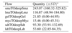
Since this model takes advantage of the dichotomy of the surface, photic ecosystem and the deep, remineralized ecosystem, let’s first look at those carbon flows that couple the two layers. There is 31 times more carbon shuttled from the surface ecosystem to the deep than visa versa. While the carbon from deep ecosystem to the surface is entirely due to the higher trophic levels (HTL), the sources of the carbon being shuttled to the deep are more diverse.
The data collected by the CCE LTER deployment cruises comes from a variety of rate measurements taken over a four day cycle. Each of these cycles ($n=7$) aim to capture a snapshot of the ecosystem at that particular location (each cycle is deployed in a different area within the upwelling region). Through this approach, data is collected for the ecosystem present under a diverse set of conditions (e.g. nutrient concentrations, temperature, mixed-layer depth, Fe-light co-limitation, etc.) which should provide adequate information for a space-for-time analysis (see Lester et al. 2014 for an introduction). To begin with, let’s first look at an single cycle in isolation.
Cycle 3
The Inverse Modeling technique provides an estimation of the fluxes between any two compartments, which can provide some interesting derived quantities (second order) that are virtually impossible to measure in situ. For example, Gross Growth Efficiencies are critical to our understanding of the marine trophic cascade and the organic carbon pools (Figure 3).
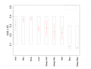
While microzoa (MIC) are the dominant heterotrophic plankton class by biomass ($556 \pm 95\ mg\ C m^{-2}$) and by observed grazing rates ($717 \pm 200\ mg\ C m^{-2}d^{-1}$), these plankton are non-vertically migrating and therefore cannot directly export carbon to depth. Instead it is the small mesozoa (SMZ) who are capable of vertical migration and whose grazing rates are greater than the grazing rates of large mesozoa (LMZ) ($146 \pm 67$ and $51 \pm 18\ mg\ C m^{-2}d^{-1}$, respectively). The SMZ constitute the primary flow of carbon from the surface to depth accounting for 45\% of net carbon export to the deep ecosystem (Table 1).
In addition to the carbon shuttled by the diurnal migration of SMZ and LMZ, sinking detritus is a substantial fraction of the total with small detritus (SDT) and large detritus (LDT) constituting $17\%$ and $10\%$ of the total, respectively.
To place the detritus terms into context, we can look at the fates, and the relationships between those fates, of both the large and small detritus pools. The fate of SDT is comparably simple to that of the LDT since there are just four pathways for the carbon to take (while LDT has six pathways). SDT can (A) sink to depth, (B) be grazed on by HNF, (C) be grazed on by MIC, or (D) decompose into DOC. Using these flows, Figure 5 shows a heat map of how the flows covary within the solution space of the model.

The analysis indicates that the HNF control the fate of the SDT within this ecosystem. When more small detritus is grazed on by the HNF, the three other fluxes tend to decrease as indicated by the negative correlation coefficient. A possible explanation for this behaviour is based on the composition of the heterotrophic plankton community in the respective areas.
For example, cycle 1 results show a similar pattern of control for the flows away from SDT, but the controlling plankter has changed. While HNF control the fate of SDT in cycle 3 (Figure 5), MIC are the controller in cycle 1 (data not shown). This also appears to correlate with an increase in total flux of $7\%$ through the MIC compartment relative to GPP (i.e. $\sum{MIC}/GPP$). A more thorough comparison including the data from all the cycles is required before conclusions can be drawn.
After running the same analysis for the LDT pool in cycle 3, we find that it is the MIC who exerts control over the fate of the LDT (Figure 6). This result may be due to the relative abundance of the MIC over those organisms that can ingest LDT once the HNF are subtracted (since HNF are required to apply pressure on the SDT).

Multi cycle
An important goal of this project is to integrate a range of measurements across a diverse and heterogeneous region. To that end, comparing the results of the model across the range of cycles is critical and necessary. Comparing observed values against the model output provides a reasonable check on both the model and/or the measurements themselves. Summarized in Figure 7, the resultant solutions for cycle’s 1, 3, 4, 5, 6 and 7 are plotted for (A) NPP, (B) LMZ grazing, (C) MIC grazing and (D) SMZ grazing.
Overall the measured values and the model output agree to within about a SD (their agreement could be measured as distance from the point to the 1:1 dashed line), but certain trends are evident. The NPP values tend to be higher for the model than what was measured in the field (panel A), this could be explained as either a bias in the model or that the protocol used to measure NPP is biased downwards. Without further information there is no a priori way to determine the cause.
Similar trends also exist within the grazing fluxes which the implication of which will be left to a future point in time.

Future Work
As with any model, the results are only as reliable as the data driving it. Since ecosystems are notoriously under-constrained problems in that the number of degrees of freedom allowed a solution, $\vec{x}$, by the model is large, an accurate analysis of the model is essential. One aspect of this analysis will include looking at the sensitivity of the output based on our \emph{a priori} assumptions of the ecosystem such as maximum and minimum grazing rates, gross growth efficiencies and temperature dependencies.
Since the model generates possible solutions by picking pseudo-random points within the solution space, an accurate sampling of this space is essential to compiling accurate results. To do this, the model must run long enough to fully sample the space while also being tuned to run in a reasonable amount of time and in an unbiased way. To put these considerations into context, recall that within the model just 37 equations (23 exact and 14 approximate) and 80 inequalities are available to constrain a solution in a 103 dimensional space. The size of any particular solution space is quite large so sampling it accurately requires many millions of CPU cycles.

Once the model is properly tuned and understood, statistical tools for analyzing the results will poise opportunities to deepen our understanding of the ecosystem. Through the use of data clustering–such as k-means–it may be possible to generalize the spectrum of solutions into useful categories based on functional understandings (third order analysis). For example, Figure 8 shows a h-cluster of 25 randomly sampled solutions where each solution’s distance from other solutions is plotted. The length of the connecting segments indicates how similar the corresponding solutions are to one another. So two solutions separated by long segments are essentially very different solutions. The bifurcation of the dendrogram suggests that there exist two, statistically distinct, branches of solutions (Labeled 1 and 2). While only speculative at this point, perhaps branch 1 solutions are ones for a deep ecosystem controlled by passive carbon flux whereas the other branch contains solutions that are controlled by vertical migrators. More analysis is certainly needed but the possibility is stimulating.
The method to determine the distance between the solutions for the above clustering approaches is to calculate the euclidian distance between the vector solutions $\vec{x}$ as shown in the equation below. While this does weight all the flows linearly and has known issues with high-dimensional data (Aggarwal 2001), it is the most straightforward metric for the analysis. A more rigorous treatment is called for.
$d(\vec{x}’, \vec{x}) = \sum_{i=1}^{103}(x’_i-x_i)^2$
With this model, a specific question will be asked in addition any other’s that arise de novo. Fish and vertically migrating plankton species are known carbon exporters by grazing on food sources in the surface waters and then migrating down in the water column on a, typically, diurnal scale (Davison et al. 2013). While estimates have been made in the past, measuring the resulting carbon export directly has been challenging; and yet it represents an important mechanism within the biological pump and carbon sequestration.
References



One thought on “End of the Semester”
Comments are closed.